Data Analyst Project 3¶

Data Wrangle (Retrieve, Analyze and Clean) OpenStreetMaps Data from the City of Dresden

by Benjamin Söllner, benjamin.soellner@gmail.com

based on the Udacity.com Data Wrangling With MongoDB

The city of Dresden as a JSON object illustration

Abstract¶

This paper describes describes the process of downloading, analyzing and cleaning of an OpenStreet Map data set of my former home town as a student: Dresden, a state capital in eastern Germany, a baroque town beautifully located on the board of the river Elbe and town home to a high-tech conglomerate from the micro-electronics sector called Silicon Saxony.

In this paper, first, the pipeline (and python script) to perform retrieval, analysis and cleaning of the data is introduced (chapters Approach) and results of the analysis stage are presented (chapter Overview of the Data). During the analysis, interesting facts of Dresden are uncovered, like the most popular religion, sport, beer, cuisine or leisure activity.

For the cleaning stage (chapter Problems Encountered in the Map), canonicalizing phone numbers present in the data set and unifying cuisine classifications where the challenge of choice. Some other cleaning techniques like cleaning street names and post codes where tried, but proved not fruitful. The paper is finally concluded with some further ideas for data set cleaning (chapter Other Ideas about the Data Set).

The Approach¶

I implemented retrieving / storing / analysing and cleaning in a python script. The script can be used like this:

# python project.py
Usage:
  python project.py -d    Download & unpack bz2 file to OSM file (experimental)
  python project.py -p    Process OSM file and write JSON file
  python project.py -w    Write JSON file to MongoDB
  python project.py -z    Download and install the zipcode helpers"
  python project.py -f    Audit format / structure of data
  python project.py -s    Audit statistics of data
  python project.py -q    Audit quality of data
  python project.py -Z    Audit quality of data: Zipcodes - (see -z option)
  python project.py -c    Clean data in MongoDB
  python project.py -C    Clean data debug mode - don't actually write to DB

Different options can be combined, so python project.py -dpwfsqc will do the whole round trip. During the process, I re-used most of the code and data format developed during the "Data Wrangling With MongoDB" Udacity course. For example, the data format used for storing the data (-p and -w option) is completely based on Lesson 6 - with some fine-tuning.

Some output of the script is shown on the terminal, some is written to local files. If a file is written, this is indicated in the terminal output. A sample of the script's terminal output is included in the output_*.txt files included in the submission.

Data Format¶

Try it out: Use python project.py -f to obtain the data for this chapter. This is a long-running process which might take a few hours to complete! There is an output file written to Project/data/audit_format_map.csv which can be beautified into an Excel spreadsheet.

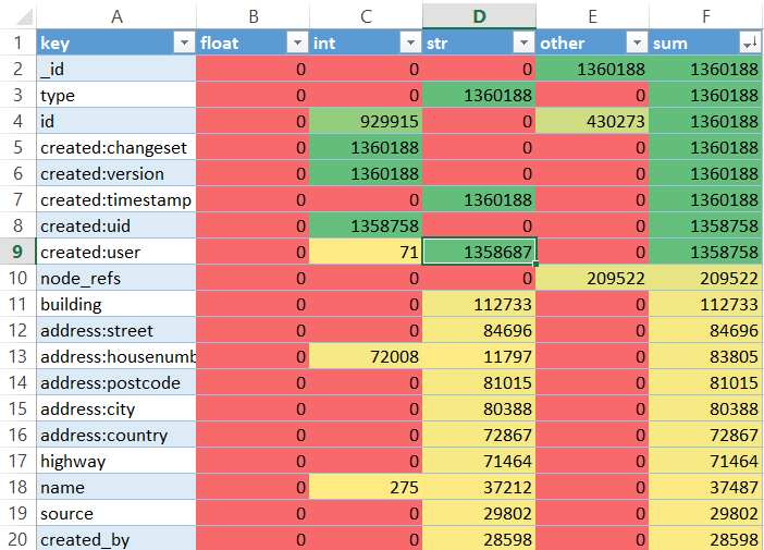
A picture of the excel spreadsheet audit_format.xlsx

First, the data format was audited, which consisted of going through all the documents and aggregating the occurence of any attributes and the prevalence of their types (string, integer, float and other). For this, batches of 1000 documents each are retrieved from the collection and each combed through by the python code while a Python Dataframe keeps track of the counters. Since there are 1,360,000 elements, this process takes many hours; an alternative would be to run the query natively in JavaScript code on the MongoDB shell or to issue the command as a BSON command.

The overview of the format showed no obvious big problems with the data at first glance but provided some valuable insights:

One area of improvement could be the phone number, which is scattered across multiple data fields (address:phone, phone and phone_mobile) and was identified as a potential candidate for cleaning (see Auditing Phone Numbers and Cleaning Phone Numbers).
Some values are present in the dataset as sometimes string, othertimes numeric: The XML parsing process takes care that each value is, whenever parsable, stored as integer or float. For attributes like street numbers, mixed occurences may be in the data set.
This automatic parsing of int or float turned out to be not always useful: a problem are leading zeros which in certain cases hold semantics. For german phone numbers, a leading zero signifies the start of an area code (0) or the start of a country code (00). For german postcodes, a leading zero in a postcode represents the german state of Saxony. As an outcome of this insight, I changed the parsing routine of the XML data to only parse values as numeric, if they do not contain a leading zero (not s.startswith("0"))
I checked some of the lesser-common values for sanity. E.g., there is a parameter dogshit which appears three times. As it turns out, this is not a prank of some map editors, who document dog feces they find in the area, but an indication about whether a public trash can contains a dispenser of plastic bags for relevant situations.

Overview of the Data¶

Try it out: Use python project.py -s to obtain the data for this chapter. See Sample Output in file Project/output_project.py_-s.txt.

A couple of basic MongoDB queries were run to explore the data set based on the knowledge of its format from the previous chapter. The queries produce mostly rankings of values for certain data fields. Some of them are subsequently also visualized in a ggplot graph (png file) relying on the skill set gained in Udacity's Intro to Data Science course, Lesson 4: Data Visualization while not too much effort was put in making the graphs look particularily beautiful. The graphs are located in Project/data/stats_*.png.

Filesize, Number of Nodes and Ways¶

The total file size of the OSM export is 281.778.428 Bytes, there are 208813 nodes and 1146807 ways in the dataset.

from Project.notebook_stub import project_coll
import pprint

# Query used - see function Project.audit_stats_map.stats_general
pipeline = [
        {"$group": {"_id": "$type", "count": {"$sum": 1}}},
        {"$match": {"_id": {"$in": ["node", "way"]}}}
    ]
l = list(project_coll.aggregate(pipeline))
pprint.pprint(l)

[{u'_id': u'way', u'count': 209356}, {u'_id': u'node', u'count': 1148321}]

Users Involved¶

There were about 1634 users involved in creating the data set, the top 10 of all users accounts for 40% of the created data. There is no direct evidence from the user name that any of them are bot-like users. This could be determined by further research. Many users (over 60%) have made less than 10 entries.

from Project.notebook_stub import project_coll
import pprint

# Query used - see function: Project.audit_stats_map.stats_users(...):
pipeline = [
        {"$match": {"created.user": {"$exists": True}}},
        {"$group": {"_id": "$created.user", "count": {"$sum": 1}}},
        {"$sort": {"count": -1}}
    ]
l = list(project_coll.aggregate(pipeline))
print str(len(l)) + " users were involved:"
pprint.pprint(l[1:5]+["..."]+l[-5:])

1634 users were involved:
[{u'_id': u'Wolle DD', u'count': 145807},
 {u'_id': u'NESDD', u'count': 79159},
 {u'_id': u'Thomas8122', u'count': 75621},
 {u'_id': u'stw1701', u'count': 57403},
 '...',
 {u'_id': u'chkr', u'count': 1},
 {u'_id': u'The King', u'count': 1},
 {u'_id': u'mowsw', u'count': 1},
 {u'_id': u'kicherschleife', u'count': 1},
 {u'_id': u'choess', u'count': 1}]

Types of Amenities¶

The attribute amenity inspired me to do further research in which kind of buildings / objects / facilities are stored in the Open Street Map data in larger quantities in order to do more detailed research on those objects. Especially Restaurants, Pubs and Churches / Places of Worship were investigated further (as can be seen below).

from Project.notebook_stub import project_coll
import pprint

# Query used - see function: Project.audit_stats_map.stats_amenities(...):
pipeline = [
        {"$match": {"amenity": {"$exists": True}}},
        {"$group": {"_id": "$amenity", "count": {"$sum": 1}}},
        {"$sort": {"count": -1}}
    ]
l = list(project_coll.aggregate(pipeline))
pprint.pprint(l[1:10]+['...'])

[{u'_id': u'parking', u'count': 2689},
 {u'_id': u'bicycle_parking', u'count': 959},
 {u'_id': u'recycling', u'count': 892},
 {u'_id': u'post_box', u'count': 793},
 {u'_id': u'restaurant', u'count': 684},
 {u'_id': u'vending_machine', u'count': 616},
 {u'_id': u'waste_basket', u'count': 536},
 {u'_id': u'fast_food', u'count': 330},
 {u'_id': u'telephone', u'count': 329},
 '...']

Popular Leisure Activities¶

The attribute leisure shows the types of leisure activities one can do in Dresden and inspired me to invesigate more on popular sports in the city (leisure=sports_center or leisure=stadium).

from Project.notebook_stub import project_coll
import pprint

# Query used - see function: Project.audit_stats_map.stats_amenities(...):
pipeline = [
        {"$match": {"leisure": {"$exists": True}}},
        {"$group": {"_id": "$leisure", "count": {"$sum": 1}}},
        {"$sort": {"count": -1}}
    ]
l = list(project_coll.aggregate(pipeline))
pprint.pprint(l[1:10]+['...'])

[{u'_id': u'pitch', u'count': 575},
 {u'_id': u'park', u'count': 431},
 {u'_id': u'sports_centre', u'count': 193},
 {u'_id': u'garden', u'count': 190},
 {u'_id': u'swimming_pool', u'count': 108},
 {u'_id': u'track', u'count': 48},
 {u'_id': u'dance', u'count': 23},
 {u'_id': u'water_park', u'count': 22},
 {u'_id': u'stadium', u'count': 19},
 '...']

Religions in Places of Worship¶

Grouping and sorting by the occurences of the religion attribute for all amenities classified as place_of_worship or community_center gives us an indication, how prevalent religions are in our city: obviously, christian is the most prevalent here.

from Project.notebook_stub import project_coll
import pprint

# Query used - see function: Project.audit_stats_map.stats_religions(...):
pipeline = [
        {"$match": {"amenity":{"$in": ["place_of_worship","community_center"]}}},
        {"$group": {"_id": "$religion", "count": {"$sum": 1}}},
        {"$sort": {"count": -1}}
    ]
l = list(project_coll.aggregate(pipeline))
pprint.pprint(l)

[{u'_id': u'christian', u'count': 140},
 {u'_id': u'muslim', u'count': 3},
 {u'_id': u'buddhist', u'count': 2},
 {u'_id': None, u'count': 2},
 {u'_id': u'jewish', u'count': 2},
 {u'_id': u'multifaith', u'count': 1}]

Cuisines in Restaurants¶

We can list the types of cuisines in restaurants (elements with attribute amenity matching restaurant) and sort them in decending order. We can notice certain inconsistencies or overlaps in the classifications of this data: e.g., a kebab cuisine may very well be also classified as an arab cuisine or may, in fact a sub- or super-classification of this cuisine. One could, e.g., eliminate or cluster together especially occurences of cuisines which are less common, but Without having a formal taxonomy of all cuisines, I decided that is probably best to leave the data as-is in order to not sacrifice preciseness for consistency.

from Project.notebook_stub import project_coll
import pprint

# Query used - see function: Project.audit_stats_map.stats_cuisines(...):
pipeline = [
        {"$match": {"amenity": "restaurant"}},
        {"$group": {"_id": "$cuisine", "count": {"$sum": 1}}},
        {"$sort": {"count": -1}}
    ]
l = list(project_coll.aggregate(pipeline))
pprint.pprint(l[1:10]+['...'])

[{u'_id': u'german', u'count': 66},
 {u'_id': u'regional', u'count': 56},
 {u'_id': u'italian', u'count': 52},
 {u'_id': u'greek', u'count': 28},
 {u'_id': u'asian', u'count': 28},
 {u'_id': u'pizza', u'count': 17},
 {u'_id': u'chinese', u'count': 12},
 {u'_id': u'international', u'count': 11},
 {u'_id': u'indian', u'count': 11},
 '...']

Beers in Pubs¶

Germans do love their beers and the dataset shows that certain pubs, restaurants or bars are sponsored by certain beer brands (often advertised on the pubs entrance). We can analyze the prevalence of beer brands by grouping and sorting by occurence of the attribute brewery for all the amenities classified as respective establishment. Most popular are Radeberger, a very popular local beer, Feldschlösschen, a swiss beer and Dresdner Felsenkeller, a very local and niche-sort-of beer.

from Project.notebook_stub import project_coll
import pprint

# Query used - see function: Project.audit_stats_map.stats_beers(...):
pipeline = [
        {"$match": {"amenity": {"$in":["pub","bar","restaurant"]}}},
        {"$group": {"_id": "$brewery", "count": {"$sum": 1}}},
        {"$sort": {"count": -1}}
    ]
l = list(project_coll.aggregate(pipeline))
pprint.pprint(l)

[{u'_id': None, u'count': 867},
 {u'_id': u'Radeberger', u'count': 10},
 {u'_id': u'Feldschl\xf6\xdfchen', u'count': 3},
 {u'_id': u'Dresdner Felsenkeller', u'count': 3},
 {u'_id': u'Warsteiner', u'count': 2},
 {u'_id': u'Rechenberger', u'count': 2},
 {u'_id': u'Feldschl\xf6\xdfchen;Schwarzer Steiger', u'count': 2},
 {u'_id': u'Einsiedler', u'count': 1},
 {u'_id': u'Eibauer', u'count': 1},
 {u'_id': u'Freiberger', u'count': 1},
 {u'_id': u'Freiberger;Jever;Astra;Lech;Tyskie;B\xf6hmisch Brauhaus',
  u'count': 1},
 {u'_id': u'Kulmbacher', u'count': 1},
 {u'_id': u"Neustadt Helles;Lenin's Hanf", u'count': 1},
 {u'_id': u'Feldschl\xf6\xdfchen;Paulaner;Schwarzer Steiger', u'count': 1},
 {u'_id': u'Radeberger;Eibauer', u'count': 1}]

Popular Sports¶

To investigate, which sports are popular, we can group and sort by the (occurence of the) sport attribute for all elements classified as sports_centre or stadium in their leisure attribute. Unsurprisingly for a german city, we notice that 9pin (bowling) and soccer are the most popular sports, followed by climbing, an activity very much enjoyed by people in Dresden, presumably because of the close-by sand-stone mountains of the national park Sächsische Schweiz.

from Project.notebook_stub import project_coll
import pprint

# Query used - see function: Project.audit_stats_map.stats_sports(...):
pipeline = [
        {"$match": {"leisure": {"$in": ["sports_centre","stadium"]}}},
        {"$group": {"_id": "$sport", "count": {"$sum": 1}}},
        {"$sort": {"count": -1}}
    ]
l = list(project_coll.aggregate(pipeline))
pprint.pprint(l[1:5]+['...'])

[{u'_id': u'multi', u'count': 55},
 {u'_id': u'9pin', u'count': 5},
 {u'_id': u'soccer', u'count': 5},
 {u'_id': u'climbing', u'count': 4},
 '...']

Where to Dance in Dresden¶

I am a passionate social dancer, so a list of dance schools in Dresden should not be abscent from this investigation. We can quickly grab all elements which have the leisure attribute set to dancing.

from Project.notebook_stub import project_coll
import pprint

# Query used - see function: Project.audit_stats_map.stats_dances(...):
l = list(project_coll.distinct("name", {"leisure": "dance"}))
pprint.pprint(l[1:10]+['...'])

[u'Tanzschule Graf',
 u'Tanzschule Weise',
 u'tres tangos',
 u'Tango im Salon',
 u'Studio24',
 u'La Academia Tango',
 u'Tanzschule Herrmann-Nebl',
 u'Tanzstudio Sandana',
 u'TSC Casino Dresden e.V.',
 '...']

Problems Encountered in the Map / Data Quality¶

Try it out: Use python project.py -q to obtain the data from this chapter. See Sample Output in file Project/output_project.py_-q.txt. The script also writes a CSV file to Project/data/audit_buildings.csv, which is also beautified into a Excel File.

Leading Zeros¶

As already discussed, during the parsing stage, we are using an optimistic approach of parsing any numerical value as integer or float, if it is parsable as such. However, we noticed that we should not do this, if leading zeros are present as those hold semantics for phone numbers and zip codes. Otherwise, this cleaning approach gives us a much smaller representation of the data in MongoDB and in-memory.

Normalizing / Cleaning Cuisines¶

As hinted in section Cuisines in Restaurant, classification of cuisines is inconsistent. There are two problems with this value:

There are multiple values separated by ';' which makes the parameter hard to parse. We overcome this by creating a parameter cuisineTag which stores the cuisine classifications as an array:

db.eval('''db.osmnodes.find({
                      "cuisine": {"$exists": true},
                      "amenity": "restaurant"
                  }).snapshot().forEach(function(val, idx) {
                      val.cuisineTags = val.cuisine.split(';');
                      db.osmnodes.save(val)
                  })
           ''')

Some values are inconsistently used; therefore, we unify them with a mapping table and a subsequent MongoDB update:

cuisines_synonyms = {
    'german': ['regional', 'schnitzel', 'buschenschank'],
    'portuguese': ['Portugiesisches_Restaurant_&_Weinbar'],
    'italian': ['pizza', 'pasta'],
    'mediterranean': ['fish', 'seafood'],
    'japanese': ['sushi'],
    'turkish': ['kebab'],
    'american': ['steak_house']
  }
# not mapped:
# greek, asian, chinese, indian, international, vietnamese, thai, spanish, arabic
# sudanese, russian, korean, hungarian, syrian, vegan, soup, croatian, african
# balkan, mexican, french, cuban, lebanese

for target in cuisines_synonyms:
  db.osmnodes.update( {
      "cuisine": {"$exists": True},
      "amenity": "restaurant",
      "cuisineTags": {"$in": cuisines_synonyms[target]}
    }, {
      "$pullAll": { "cusineTags": cuisines_synonyms[target] },
      "$addToSet": { "cuisineTags": [ target ] }
    }, multi=False )

This allows us to convert a restaurant with the MongoDB representation

{..., "cuisine": "pizza;kebab", ...}

to the alternative representation

{..., "cuisine": "pizza;kebab", "cuisineTag": ["italian", "turkish"], ...}

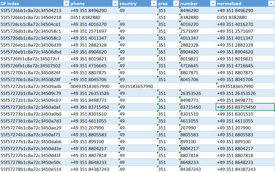
Auditing Phone Numbers¶

Phone re scattered over different attributes (address.phone, phone and mobile_phone) and come in different styles of formating (like +49 351 123 45 vs. 0049-351-12345). First, we retrieve a list of all phone numbers. With the goal in mind to later store the normalized phone number back into the attribute phone, this value has to be read first, and only if it is empty, mobile_phone or address.phone should be used.

from Project.notebook_stub import project_coll

# Query used - see function: Project.audit_quality_map.audit_phone_numbers(...):
pipeline = [
        {"$match": {"$or": [
                {"phone": {"$exists": True}},
                {"mobile_phone": {"$exists": True}},
                {"address.phone": {"$exists": True}}
            ]}},
        {"$project": {
                "_id": 1,
                "phone": {"$ifNull": ["$phone", {"$ifNull": ["$mobile_phone", "$address.phone"]}]}
            }}
    ]
l = project_coll.aggregate(pipeline)

# Output too long... See the file Project/output_project.py_-q.txt

Cleaning Phone Numbers¶

Try it out: Use python project.py -C to clean in debug mode. See Sample Output in file Project/output_project.py_-C.txt. The script also writes a CSV file to Project/data/clean_phones.csv, which is also beautified into a Excel File.

Cleaning the phone numbers involves:

unifying the different phone attributes (phone, address.phone and mobile_phone) - this is already taken care by extracting the phone numbers during the audit stage
if possible, canonicalizing the phone number notations by parsing them using a regular expression:

phone_regex = re.compile(ur'^(\(?([\+|\*]|00) *(?P<country>[1-9][0-9]*)\)?)?' +  # country code
                         ur'[ \/\-\.]*\(?0?\)?[ \/\-\.]*' +  # separator
                         ur'(\(0?(?P<area1>[1-9][0-9 ]*)\)|0?(?P<area2>[1-9][0-9]*))?' +  # area code
                         ur'[ \/\-\.]*' +  # separator
                         ur'(?P<number>([0-9]+ *[\/\-.]? *)*)$', # number
                         re.UNICODE)

The regular expression is resilient to various separators ("/", "-", " ", "(0)") and bracket notation of phone numbers. It is not resilient for some unicode characters or written lists of phone numbers which are designed to be interpreted by humans (using separators like ",", "/-" or "oder" lit. or). During the cleaning stage, an output is written which phone numbers could not be parsed. This contains only a tiny fraction of phone numbers (9 or 0.5%) which would be easily cleanable by hand.

The following objects couldn't be parsed:
                                                 normalized
55f57294b1c8a72c34523897           +49 35207 81429 or 81469
55f57299b1c8a72c345272cd  +49 351 8386837, +49 176 67032256
55f572c2b1c8a72c34546689                      0351 4810426
55f572c3b1c8a72c34546829         +49 351 8902284 or 2525375
55f572fdb1c8a72c34574963   +49 351 4706625, +49 351 0350602
55f573bdb1c8a72c3460bdb3                +49 351 87?44?44?00
55f573bdb1c8a72c3460c066         0162 2648953, 0162 2439168
55f573edb1c8a72c346304b1           03512038973, 03512015831
55f5740eb1c8a72c34649008                0351 4455193 / -118

If the phone number was parsable, the country code, area code and rest of the phone number are separated and subsequently strung together to a canonical form. The data to be transformed is stored into a Pandas Dataframe. By using the option -C instead of -c the execution of the transformation can be surpressed and the Dataframe instead be written to a CSV file which might be further beautified into an Excel File in order to test or debug the transformation before writing it to the database with the -c option.

A screenshot of the Excel file

Auditing Street Names (Spoiler Alert: No Cleaning Necessary)¶

Auditing the map's street names analogous to how it was done in the Data Wrangling course was done as follows: Check, whether 'weird' street names occur, which do not end on a suffix like street (in German -straße or Straße, depending on whether it is a compound word or not). It is assumed that then, they would most likely end in an abbreviation like str.. For this we use a regular expression querying all streets not ending with a particular suffix like [Ss]traße (street), [Ww]eg (way) etc. This is accomplished by a chain of "negative lookbehind" expressions ((?<!...)) which must all in sequence evaluate to "true" in order to flag a street name as non-conforming.

from Project.notebook_stub import project_coll

# Query used - see function: Project.audit_quality_map.audit_streets(...):
expectedStreetPattern = \
    u"^.*(?<![Ss]tra\u00dfe)(?<![Ww]eg)(?<![Aa]llee)(?<![Rr]ing)(?<![Bb]erg)" + \
    u"(?<![Pp]ark)(?<![Hh]\u00f6he)(?<![Pp]latz)(?<![Bb]r\u00fccke)(?<![Gg]rund)$"
l = list(project_coll.distinct("name", {
                    "type": "way",
                    "name": {"$regex": expectedStreetPattern}
                }))
# Output too long... See the file Project/output_project.py_-q.txt

Skimming through the list, it was noticable that the nature of the german language (and how in Germany streetnames work) results in the fact, that there are many small places without a suffix like "street" but "their own thing" (like Am Hang lit. 'At The Slope', Beerenhut lit. 'Berry Hat', Im Grunde lit. 'In The Ground'). The street names can therefore not be processed just by looking at the suffixes - I tried something different...

Cross Auditing Street Names with Street Addresses (Spoiler Alert: No Cleaning Necessary)¶

I did not want to trust the street names of the data set fully yet. Next, I tried figuring out if street names of buildings were consistent with street names of objects in close proximity. Therefore, a JavaScript query is run directly on the database server returning all buildings with the objects nearby having an address.street parameter. This should allow us to cross-audit if objects in close proximity do have the same street names.

from Project.notebook_stub import project_db

# Query used - see function: Project.audit_quality_map.audit_buildings(...):
buildings_with_streets = project_db.eval('''
            db.osmnodes.ensureIndex({pos:"2dsphere"});
            result = [];
            db.osmnodes.find(
                    {"building": {"$exists": true}, "address.street": {"$exists": true}, "pos": {"$exists": true}},
                    {"address.street": "", "pos": ""}
                ).forEach(function(val, idx) {
                    val.nearby = db.osmnodes.distinct("address.street",
                            {"_id": {"$ne": val._id}, "pos": {"$near": {"$geometry": {"type": "Point", "coordinates": val.pos}, "$maxDistance": 50, "$minDistance": 0}}}
                        );
                    result.push(val);
                })
            return result;
        ''')

# Output too long... See the file Project/output_project.py_-q.txt

The resulting objects are then iterated through and the best and worst fitting nearby street name are identified each using the Levenshtein distance. For each object, a row is created in a DataFrame which is subsequently exported to a csv file Project/data/audit_buildings.csv that was manually beautified into an Excel File.

Screenshot of the Excel File

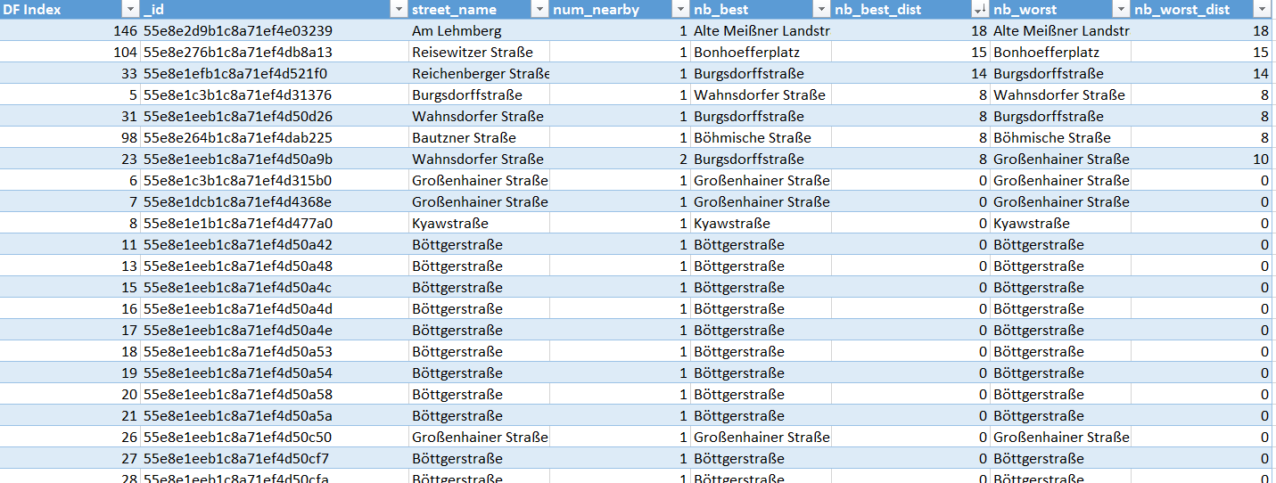
As can be seen, street names of nearby objects mostly match those of the building itself (Levenshtein distance is zero). If they deviate greatly, they are totally different street names in the same area and not just "typos" or non-conforming abbreviations.

Auditing Zip Codes (Spoiler Alert: No Cleaning Necessary)¶

Try it out: Use python project.py -Z which runs the auditing script for zipcodes. See Sample Output in file Project/output_project.py_-Z.txt. To be able to run this script correctly, the zipcode data from Geonames.org needs to be downloaded and installed first using the -z option (see output in `Project/output_project.py_-Z.txt).

This part of the auditing process makes use of an additional at Geonames.org to resolve and audit the zip codes in the data set. During the "installation process" (option -z) the zipcode data (provided as a tab-separated file) is downloaded and, line-by-line, stored to a (separate) MongoDB collection. However, we are only interested "zipcode" (2) and "place" (3)

During the auditing stage (option -Z) we first get a list of all used zipcode using the following query:

pipeline = [
            { "$match": {"address.postcode": {"$exists": 1}} },
            { "$group": {"_id": "$address.postcode", "count": {"$sum": 1}} },
            { "$sort": {"count": 1} }
        ]

The zipcodes are then all looked up in the zipcode collection using the $in-operator. The data obtained is joined back into the original result.

zipcodeObjects = zipcodeColl.find( {"zipcode": {"$in": [z["_id"] for z in zipcodeList]}} )

The following output shows that there the lesser used zipcodes are from the Dresden metropolitan area, not Dresden itself:

from Project.audit_zipcode_map import audit_zipcode_map
from Project.notebook_stub import project_server, project_port
import pprint

zipcodeJoined = audit_zipcode_map(project_server, project_port, quiet=True)
pprint.pprint(zipcodeJoined[1:10]+['...'])

[{u'_id': u'01847', u'count': 2, 'place': u'Lohmen'},
 {u'_id': u'01896', u'count': 17, 'place': u'Pulsnitz'},
 {u'_id': u'01665', u'count': 18, 'place': u'Diera-Zehren'},
 {u'_id': u'01689', u'count': 63, 'place': u'Weinb\xf6hla'},
 {u'_id': u'01833', u'count': 93, 'place': u'Stolpen'},
 {u'_id': u'01477', u'count': 134, 'place': u'Arnsdorf'},
 {u'_id': u'01737', u'count': 165, 'place': u'Tharandt'},
 {u'_id': u'01471', u'count': 325, 'place': u'Radeburg'},
 {u'_id': u'01796', u'count': 516, 'place': u'Pirna'},
 '...']

Other Ideas about the Data Set¶

Auditing City Names for Correctness and Completeness¶

The Geonames.org data could help us to validate the entered city names or add them, where missing. One could compare the address.city attribute of any OSM element with all of the 4 hierarchically names of the Geonames.org document which belongs to the zipcode referred by address.postcode.

If no address.city is present in the OSM element at all, the lowestmost value in the Geonames.org hieararchy could be added and the data therefore enhanced.
If the value of the OSM element does not match any name of the Geonames.org data, the element could be flagged for manual processing.

Cost: Relatively easily implementable, however, out of scope for this project. We should, however, strive for implementing the related query in native BSON code in order to not hit the database with every zipcode-to-Geonames-element mapping request for each OSM element.

Benefit: Potentially high, depending on how many cities are not entered at all (quick win) or entered correctly (some additional manual work required).

Cuisine Taxonomy¶

The taxonomy of cuisines could be further formalized to contain super- and subsets of cuisines (e.g. each "italian" cuisine is also an "international" cuisine). With domain knowledge, coarsly classified restaurants could potentially also be sub-classified.

Cost: High, The creation of a proper cuisine-taxonomy would require substantial knowledge of the subject matter of cuisines and the subtle differences in culinary art. Also, rather than a tree-based classification, some "fusion" kitchens might overlap: any simplification or unification we carry out here comes at the cost of sacrificing detail.

Benefit: Medium-high in certain use cases, higher number of restaurants with a certain classification lets us better find the restaurant of our taste and compare various restaurants with each other.